Difference between revisions of "WebKit Users Guide"
| (69 intermediate revisions by the same user not shown) | |||
| Line 3: | Line 3: | ||
This Guide will introduce the NWK user interface (UI) and the many useful functions that enhance and support the user's experience. A separate document, the [[WebKit Authors Guide]], is under development. | This Guide will introduce the NWK user interface (UI) and the many useful functions that enhance and support the user's experience. A separate document, the [[WebKit Authors Guide]], is under development. | ||
== | == Terminology == | ||
; Model | ; Model | ||
: A system that is initialized parametrically to an start state and is sequentially clocked to produce a new state and output vector on each clock strobe. NWK supports System Dynamic (SD), Spatial and Individual-based (IB) models. Models in NWK are currently implemented either in Javascript or Java. | : A system that is initialized parametrically to an start state and is sequentially clocked to produce a new state and output vector on each clock strobe. NWK supports System Dynamic (SD), Spatial (Sp) and Individual-based (IB) models. Models in NWK are currently implemented either in Javascript or Java. | ||
;Simulation | ;Simulation | ||
: A model in execution. Simulations are managed from the UI. | : A model in execution. Simulations are managed from the UI. | ||
;Spatial (Sp) and Individual-based (IB) models | |||
: Spacial models are represented by a 2-dimensional grid of '''cells'''. At each point in time a cell assumes a '''state''' determined by the values of a set of variables. Some property of the state is visualized by the cell's color. Individual-, or '''agent'''-based models add to this a set of objects, each occupying a cell. Each object is similarly in a state visualized by color, shape and size of either a circle or square. Cells are fixed in place in a grid, with either a Cartesian or hexagonal topology, while agents move about the landscape. The edges of the landscape can either serve as fixed boundaries, or "wrap-around" horizontally and vertically to create a torus. In many simulations with fixed boundaries, agents "bounce off" the edge like a billiard ball. Agents can also bounce off each other like an ideal gas, or not interact. These choices are made by the site's author, and in some cases may be overridden. | |||
;System Dynamics (SD) | |||
: The behavior of SD models over time can often be characterized using differential or difference equations. An SD model might be the entirety of site, or might characterize the local behavior of a cell or agent in Sp and IB models. | |||
;Project | ;Project | ||
: A single unit deploying 1 or more simulations, usually employing a single Web page. Projects are specified using a '''project file''', containing [https://www.json.org/json-en.html JSON] code detailing the UI and at least providing parameters for the model. Small SD models may be specified in the project file. | : A single unit deploying 1 or more simulations, usually employing a single Web page. Projects are specified using a '''project file''', containing [https://www.json.org/json-en.html JSON] code detailing the UI and at least providing parameters for the model. Small SD models may be specified in the project file. | ||
;Site | |||
:The Webpage or pages associated with a particular project. | |||
;"Factory Settings" | ;"Factory Settings" | ||
: | : Sites are uploaded with parameters and settings determined by the author. Users may change parameters and override some setting, however factory settings can always be recovered. | ||
;"The Drawer" | ;"The Drawer" | ||
| Line 25: | Line 34: | ||
: RAMs (Runtime alterable modules) allow the author to provide the means for selecting sets of alternative algorithms used by the model. Authors may also use the RAM facility to enable a user to completely specify some model (these are called UberRAMs, or URAMs). | : RAMs (Runtime alterable modules) allow the author to provide the means for selecting sets of alternative algorithms used by the model. Authors may also use the RAM facility to enable a user to completely specify some model (these are called UberRAMs, or URAMs). | ||
; | ;NumML | ||
: | : NumML (Numerus Modeling Language) is a small, simple, domain-specific language (dsl) that serves 2 functions: 1) to specify the algorithm or model in RAMs and URAMs; and 2) to assert configuration changes to factory settings. | ||
;Analysis Platforms | ;Analysis Platforms | ||
:These are special tabs used in some | :These are special tabs used in some sites to enable such facilities as sensitivity analysis, curve fitting, MCMC, etc. | ||
;CSV | ;CSV | ||
| Line 36: | Line 45: | ||
== Platform Overview== | == Platform Overview== | ||
[[File:ui0.png|thumb|NWK User Interface]] | [[File:ui0.png|thumb|NWK User Interface]] | ||
This image shows the browser window running the sample individual-based | This image shows the browser window running the sample individual-based site [https://www.cs.oberlin.edu/~rms/wk/rps/ "Rock Paper Scissors"]. The features are all described later in this guide. | ||
;Model Inputs | ;Model Inputs | ||
:These sliders set parameters for the simulation. Changes are forwarded even while the simulation is running and may have immediate effect. | :These sliders set parameters for the simulation. Changes are forwarded even while the simulation is running and may have immediate effect. | ||
| Line 51: | Line 60: | ||
:Other displays such as Spys (showing a single current value) graphs, tables, etc. are specified in the Project file (see below). | :Other displays such as Spys (showing a single current value) graphs, tables, etc. are specified in the Project file (see below). | ||
;Side Panel | ;Side Panel | ||
:The browser page has a side panel contained in a "drawer". Use [[File:sideicon.png]] to toggle it open and closed, or pull on the lavender bar to adjust its location. The drawer contains model documentation, the preset display, a configuration window, and a log window for status reports. If the | :The browser page has a side panel contained in a "drawer". Use [[File:sideicon.png]] to toggle it open and closed, or pull on the lavender bar to adjust its location. The drawer contains model documentation, the preset display, a configuration window, and a log window for status reports. If the site uses RAMs the side panel will be wider and will contain access to RAM controls. | ||
[[File:ui2.png|thumb|UI with SD Model]] | [[File:ui2.png|thumb|UI with SD Model]] | ||
;System Dynamics | ;System Dynamics | ||
:The third image shows the | :The third image shows the model library SD [https://www.cs.oberlin.edu/~rms/wk/lotka Lotka-Volterra] site. An SD site will display the current choices for ''dt'' and integration method (Euler or RK4). These can be overridden from factory settings using the configuration window. | ||
<br clear='both'> | <br clear='both'> | ||
In subsequent sections we describe the platform's features with illustrations using one or more of the sites in the model library. The full model library can be found in the [[WebKit Examples]] document. Note that we will be looking at the Javascript model implementation only at this time, as some of the features described here are only available with this implementation. | |||
In | |||
'''When opening the Model Library examples you are advised to right-click and open the link in a new tab.''' | |||
Among the topics covered are: | |||
* User initialization of spatial and agent-based models | |||
* Presets | |||
* NumML language | |||
* RAMS and URAMS | |||
* Configuration overrides | |||
* Analysis platforms | |||
* Downloading CSVs | |||
== Model Initialization and Using Presets with Conway's Game of Life and Agents (1) == | |||
[[File:lifeinit.gif|thumb|Initializing Conway's Game of Life]] | |||
[[File:agentsinit.gif|thumb|Initializing Agents (1)]] | |||
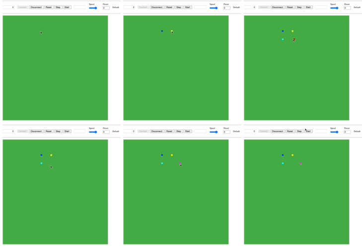
[https://www.cs.oberlin.edu/~rms/wk/life/index.html Conway's Game of Life (CGOL)] uses a 128 x 128 board with solid edge and an initial configuration consisting of the "R-pentomino". (Try it!) CGOL's model operates on a cellular automaton with 2 possible states, dead and alive. | |||
[https://www.cs.oberlin.edu/~rms/wk/agents/index.html Agents] is a very simple simulation of agents of different sizes and shapes. The space in which they are moving has elastic walls off of which the agents bounce. They also behave like an ideal gas with respect to their physical interaction. (This behavior was a choice made by the site's author.) [https://www.cs.oberlin.edu/~rms/wk/agents1/index.html Agents (1)] has the same model, only initially empty. | |||
[https://www.cs.oberlin.edu/~rms/wk/ | |||
* | With NWK you can: | ||
* Click and drag to create new initial configurations; | |||
* Save your configuration in the Presets. | * Save your configuration in the Presets. | ||
=== | === Creating new initial configurations in CGOL === | ||
To alter the initial configuration, press or click the left mouse button on any black or white cell to toggle that cell to the opposite color. If you press the mouse button, you can drag the mouse to change dragged-over cells to the new color. When done, click the '''Reset''' button once; clicking '''Run''' will execute the simulation with the new configuration, and single clicks on '''Reset''' will restore your initial configuration. Double-clicking '''Reset''' restores factory settings. | This CGOL simulation uses a Cell Matrix with black/white respectively representing dead/alive. To alter the initial configuration, '''press''' or '''click''' the left mouse button on any black or white cell to toggle that cell to the opposite color. If you press the mouse button, you can '''drag''' the mouse to change dragged-over cells to the new color. | ||
When done, '''click''' the '''Reset''' button once; clicking '''Run''' will execute the simulation with the new configuration, and single clicks on '''Reset''' will restore your initial configuration. '''Double-clicking''' '''Reset''' restores factory settings. | |||
=== Creating new initial configurations in Agents (1) === | |||
You add agents to Agents (1)'s landscape in a similar manner. '''Shift-click''' on a cell to add an agent, and continue to '''shift-click''' to rotate through cell colors. At the end of the rotation the agent will be deleted. You can also delete an agent immediately with '''alt-shift-click'''. | |||
When done, '''double-click''' '''Reset''', and then '''Run'''. To restore factory settings you must reload the page. | |||
<br clear="both"> | |||
== Preset Basics == | |||
[[File:preset.png|thumb|Preset Control]] | [[File:preset.png|thumb|Preset Control in Drawer Panel]] | ||
The Preset feature provides a quick way to save and restore a configuration, modeled on the "radio buttons" found in cars. The Preset control consists of 13 such preset buttons. Each preset label is either red or green, respectively, depending on whether or not the preset is currently assigned to a configuration. Selecting a "green" label will restore the configuration saved in that preset. Selecting a red label has no effect on the configuration. | The Preset feature provides a quick way to save and restore a configuration, modeled on the "radio buttons" found in cars. The Preset control consists of 13 such preset buttons. Each preset label is either red or green, respectively, depending on whether or not the preset is currently assigned to a configuration. Selecting a "green" label will restore the configuration saved in that preset. Selecting a red label has no effect on the configuration. | ||
'''Note that preset 0 is permanently bound to factory settings and cannot be changed'''. | '''Note that preset 0 is permanently bound to factory settings and cannot be changed'''. | ||
'''Tags.''' Each preset can be optionally given a tag; i.e., a label used to identify the settings for that preset. Simply enter the tag in the '''Tag''' text field before saving the preset. | |||
[[File:presetDemo.gif|thumb|Preset Control in Main Control Panel]] | |||
Preset and tag selection are also controlled from the main control panel, making it unnecessary to have the drawer open while shifting between different presets. The Preset control is located to the right of the Speed slider, and rotates through the available presets as it is clicked up or down. Tagged presets display their tag when selected. | |||
Configurations are saved and cleared using the '''Save/Clear/Cl All''' buttons to the right of the Preset controls. Whichever preset is selected will be affected by '''Save/Clear'''; '''Cl All''' will delete all presets (except for preset 0). | Configurations are saved and cleared using the '''Save/Clear/Cl All''' buttons to the right of the Preset controls. Whichever preset is selected will be affected by '''Save/Clear'''; '''Cl All''' will delete all presets (except for preset 0). | ||
Presets are stored in the Web browser and will be there when you return to the site. A local JSON file storing the complete current bank of presets is created using the '''Preset ↔ Local File''' controls found to the left of the Configuration window. Use stored presets as a backup, for transferring between browsers, and when you exceed the 12 user preset limit. | |||
---- | |||
Something to try | |||
Create a set of CGOL and Agent (1) initial configurations using the mouse as described and store them in presets. Test the presets by restoring the configurations. Practice using ''Save'' and ''Clear'' until you are comfortable with building configurations and storing/restoring them using the presets. | |||
---- | |||
=== One more thing about Presets === | |||
Some site include ready-made presets. These will be installed the first time you access the site. You may make changes to and save ready made presets. You can restore the factory set of ready-mades by deleting all presets and reloading the site. | |||
<br clear="both"> | |||
== Using RAMs with the Extended Game of Life 3 (EGOL3) == | |||
[[File:egol3.png|thumb|Extended Game of Life Showing RAM Panel]] | |||
[[File:egol3RAM.gif|thumb|Preset Selection Showing RAM Choices]] | |||
RAMs provide the means for changing some aspect of the site's model. Each RAM presents a set of alternatives, including a Display or Default alternative that is part of the factory settings. An Alternative may require some additional input through sliders, text fields or text areas. Space is provided so that RAMs are thoroughly documented. | |||
[https://www.biorxiv.org/content/10.1101/2022.08.30.505937v1 EGOL3] is an extension to Conway's Game of Life to 3 live states (birth, newborn and adult). The simulation has been constructed to support 4 alternate approaches to the creating the initial state, which are presented to you as a RAM with 4 alternatives. The RAM is revealed when the drawer is fully open and '''Initial State''' is selected from the RAM Selection Panel (see right). | |||
The RAM Selection Panel appears whenever a site contains one or more RAMs. Selecting a RAM replaces the content of the Documentation Window with overview documentation for the selected RAM. A new column appears topped by the RAM Alternative Selection Panel. Each alternative introduces documentation specific to that alternative and, if needed, a set of input controls (in some cases an input control such as a text area is included for reference only and cannot be edited). | |||
RAMs are powerful tools when combined with presets since the selected RAM and any input values are stored as part of the preset configuration. The factory settings for EGOL3 include 7 different initialization configurations realized mixing different main parameters, RAM alternatives and RAM parameters. You can see this in action by opening the RAM panels as shown and clicking through the 7 presets, as shown at right. | |||
The '''Display''' RAM setting is analogous to the conventional GOL we explored earlier. You can set your own initial configuration through click and drag like before. The '''Random''' setting lets you choose the probabilities for initial live cells. '''Reg6''' and '''Reg Custom''' produce diagonal stripes that repeat with, respectively, a fixed interval of 6 or with an interval between 2 and 12. | |||
---- | ---- | ||
Something to try | Something to try | ||
Make changes to the existing presets. When editing a textfield input, be sure to hit '''Enter''' when you are ready to register the change. Save configurations in any of the remaining empty presets, or override the factory presets (except for Preset 0). | |||
When you are done you can restore the initial preset configuration by deleting ''all'' presets with '''Cl All''' and then reloading. | |||
---- | ---- | ||
== Using RAMs with the Deterministic SIRS w/ Vaccination (SIRS) == | |||
SIRS is rich with RAMs with one ('''Immune to Vaccinated''') containing an alternative ('''User Input''') requiring code. This alternative lets you program how individuals in class R (recovering) are vaccinated and transferred to class V (vaccinated), as a function of model time. A set of variables that can be referenced in the code is provided. | |||
An example is contained in Preset 1. Here we choose to use apply the vaccination rate from the vaccination onset time (both set with the main input sliders) to a time determined using the RAM slider '''User 1'''. In other words, you add a shut-off time for vaccinations which has not been provided by the original model. Other possibilities for this RAM could be, for example, to let the vaccination rate decay to account for depletion of vaccine, using the '''User 1''' slider to determine the decay rate. | |||
The code used in Preset 1 is Javascript. Press the '''Compile''' button when your are ready. The '''Enlarge''' button opens a browser-wide editor window, making code entry easier. If you want to try your own User Input RAM, be sure to save in a preset or your code will be lost. | |||
== User-Defined Models (URAMs) with Sensitivity Analysis == | |||
The RAM interface makes it possible to easily implement SD simulations defined entirely by the user. An example from the model library containing 4 user-defined presets is [https://www.cs.oberlin.edu/~rms/wk/sdnumml1/index.html SD User Defined]. | |||
Such sites are initially defined only by the input and output components they support. Their operation relies on a user-defined program, specifying the model and its UI, that is entered using a RAM. The example site has a RAM with one option, that option showing a text area for the program. It also provides sufficient input and output components to support the UI needs of models implemented on the site. | |||
The example site includes 6 slider inputs, a line graph and a phase graph. Each of these 8 components need a "handle", an ID by which they can be referenced in the program. The sliders all run from 0 to 1 with 0.01 step size and have the IDs <code>Param1</code>, <code>Param2</code>..., <code>Param6</code>. The line and phase graphs are respectively given IDs <code>mainGraph</code> and <code>phaseGraph</code>. | |||
Visit the model using the link and open the '''Model Definition''' RAM. It contains a single option ('''NumML Code''') with a Code text area. Notice that, although 6 sliders were allotted, only 1 is visible in the default preset. This is a result of the UI configuration contained in the program. As you step through presets note that the input sliders appear and disappear as needed, and that slider and graph legends (names and titles) change to suit the model. | |||
Consider the code for the default Exponential Curve model: | |||
<blockquote> | |||
[[File:expocode.png|400px|Code for Exponential Model]] | |||
</blockquote> | |||
The first line consists of the string "numml". This is required to indicate that the contents are in NumML rather than Javascript. There are 2 sections: '''model''' and '''configurations'''. (Note that "//" is the comment character meaning that this line is ignored by the compiler). In the model section are 4 statements using the operator <code>@=</code>. In fact, each NumML statement uses Javascript syntax, but with 2 non-Javascript operators: <code>@=</code> and <code>#=</code>, which completely program the behavior and look and feel of the simulation. The former is used to specify the model generally in terms of differential (or difference) equations using program variables; the latter asserts properties for the visual components that fit with the particular model | |||
The first block (lines 4 - 8) consists of 3 statements defining the variable of interest, <code>Exp</code>, and one defining an auxiliary variable <code>Rate</code> used in line 4. The latter is not entirely necessary; we could instead have written line 4 as <code>deriv(Exp) @= Param1 * Exp</code>, however the style we used relates the model directly to relabeling of the <code>Param1</code> slider to <code>Rate</code> and consequently is more readable. We will continue to see this approach used in the other models in this site. | |||
<code>deriv(Exp)</code> specifies a differential equation on line 4 relating <code>Exp</code> to itself and local variable <code>Rate</code>. Line 8 binds <code>Rate</code> to <code>Param1</code>, which is the alias we assign to <code>Param1</code> on line 14. Line 5 provides an initial value for <code>Exp</code>, and line 6 links <code>Exp</code> with the line graph <code>mainGraph</code>, which displays its output.. | |||
Lines 11 through 16 use operator <code>#=</code> to detail the appearance of the input sliders and output graphs. This is mostly self- explanatory, except for the entry for <code>statsGraph</code>, which will be discussed below. This code is not required, however the result will be a generic display with 6 input sliders labeled <code>Param1</code> through <code>Param6</code>, and graphs with no labels. Note that on line 16, setting the legend for the unused sliders to an empty string hides them. | |||
Look at the remaining preset code. Preset 3, in particular, is a good example of the extent to which input sliders can be detailed. This is required because the generic slider properties do not match the value range required in the simulation. Refer to the [[NumML Language Reference]] for a complete description of the NumML language. | |||
'''If you make changes to any of these that you want to save to presets, you should compile before saving so that the compiled code will be loaded when you activate the preset.''' | |||
=== Sensitivity Analysis === | |||
One of the goals of NWK is to provide secondary platforms for optimization and analysis. To date one such platform exists to perform sensitivity analysis, primarily but not exclusively for SD models. Once again, refer to [https://www.cs.oberlin.edu/~rms/wk/sdnumml1/index.html SD User Defined] to see this in action. Open this site and click on the tab labeled '''Sensitivity'''. | |||
[[File:sens0.png|thumb|Sensitivity Analysis Platform after a run]] | |||
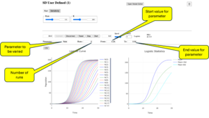
The figure show on the right shows the Sensitivity Analysis platform for the logistic model (Preset 1) after a run. There are 4 user parameters that govern the behavior as shown: | |||
* '''Parameter''': which parameter is varied (in this model it is '''Rate'''). | |||
* '''Runs''': how many runs (20); | |||
* '''From''': initial value (0.25); | |||
* '''To''': final value (0.54); | |||
Clicking '''Start''' initiates 20 runs with the '''Rate''' parameter uniformly stepping through intermediate values between 0.25 and 0.54. During this run, clicking '''Stop''' allows the most recent run to finish, allowing the process to continue by subsequently clicking '''Start'''. Alternatively, clicking '''Step''' proceeds one run at a time until the process concludes. Double-clicking '''Reset''' reinitializes the run. | |||
Results are displayed on 2 graphs, the first being identical to the one on the '''Run''' platform. To its right is a graph showing mean ± standard deviation of the point-wise variations seen in the run. | |||
Now open the '''Model Definition''' RAM and look at the code in lines 12 - 15 to see how the Sensitivity Analysis platform was programmed. The statistics display has ID ''statsGraph''. In addition to specifying a title ("Logistic Statistics"), we see the following entries: | |||
;statDat(N) | |||
:''N'' is output variable of interest | |||
;statParam(Rate) | |||
:''Rate'' is the input parameter to be varied | |||
;statRuns(20), statLo(0.25), statHi(0.54) | |||
:20 runs with ''Rate'' varying uniformly between 0.25 and 0.54 | |||
Note that except for '''statDat''', these settings are shown in textfields and merely initialize their parameters. They can be changed, and changes are saved to presets. | |||
== Configuration Overrides == | |||
[[File:config.png|thumb|Configuration Window]] | |||
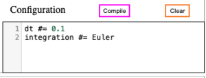
NumML statements using <code>#=</code> can be used to configure most models using the Configuration window below the Preset selection window. Shown at right is an override of the factory settings that changes the ''dt'' value and asserts Euler as the integration method. Other overrides will become available soon. | |||
<br clear="both"> | |||
== CSV Downloads == | |||
If a graph contains a '''CSV''' button, clicking that button once the graph has been filled will bring about a download of a CSV (comma separate values) file of the data from that graph. The settings used by the simulation will be recorded above the CSV header. | |||
<br clear="both"> | <br clear="both"> | ||
Latest revision as of 16:21, 11 July 2025
Numerus WebKit (NWK) is a technology for building powerful simulations that run in a Web browser. It consists of applications and APIs that support the design of models along the lines of NetLogo (NL) and Stella, but using conventional languages such as Java, JavaScript (JS) and Python.[1] These applications are deployed either from a remote server, such as Amazon Web Services (AWS) Elastic Beanstalk (AWSEB), (or, in Java mode, any other server that supports WebSockets, or in JS mode, from any conventional Web or Cloud server); alternatively, they can be run locally without using any network connectivity using a localhost server. JS development only requires text editing, and Java development can take advantage of the Eclipse J2EE (Jakarta) platform using the Apache Tomcat server.
This Guide will introduce the NWK user interface (UI) and the many useful functions that enhance and support the user's experience. A separate document, the WebKit Authors Guide, is under development.
Terminology
- Model
- A system that is initialized parametrically to an start state and is sequentially clocked to produce a new state and output vector on each clock strobe. NWK supports System Dynamic (SD), Spatial (Sp) and Individual-based (IB) models. Models in NWK are currently implemented either in Javascript or Java.
- Simulation
- A model in execution. Simulations are managed from the UI.
- Spatial (Sp) and Individual-based (IB) models
- Spacial models are represented by a 2-dimensional grid of cells. At each point in time a cell assumes a state determined by the values of a set of variables. Some property of the state is visualized by the cell's color. Individual-, or agent-based models add to this a set of objects, each occupying a cell. Each object is similarly in a state visualized by color, shape and size of either a circle or square. Cells are fixed in place in a grid, with either a Cartesian or hexagonal topology, while agents move about the landscape. The edges of the landscape can either serve as fixed boundaries, or "wrap-around" horizontally and vertically to create a torus. In many simulations with fixed boundaries, agents "bounce off" the edge like a billiard ball. Agents can also bounce off each other like an ideal gas, or not interact. These choices are made by the site's author, and in some cases may be overridden.
- System Dynamics (SD)
- The behavior of SD models over time can often be characterized using differential or difference equations. An SD model might be the entirety of site, or might characterize the local behavior of a cell or agent in Sp and IB models.
- Project
- A single unit deploying 1 or more simulations, usually employing a single Web page. Projects are specified using a project file, containing JSON code detailing the UI and at least providing parameters for the model. Small SD models may be specified in the project file.
- Site
- The Webpage or pages associated with a particular project.
- "Factory Settings"
- Sites are uploaded with parameters and settings determined by the author. Users may change parameters and override some setting, however factory settings can always be recovered.
- "The Drawer"
- The NWK screen has a sliding partition on the right-hand side, controlled by the user, that reveals documentation and other features detailed below when slid leftward.
- Presets
- NWK provides a storage facility to record and recall various choices for settings and parameters. The presets are like "radio buttons" selecting various alternative sets of configurations.
- RAMs
- RAMs (Runtime alterable modules) allow the author to provide the means for selecting sets of alternative algorithms used by the model. Authors may also use the RAM facility to enable a user to completely specify some model (these are called UberRAMs, or URAMs).
- NumML
- NumML (Numerus Modeling Language) is a small, simple, domain-specific language (dsl) that serves 2 functions: 1) to specify the algorithm or model in RAMs and URAMs; and 2) to assert configuration changes to factory settings.
- Analysis Platforms
- These are special tabs used in some sites to enable such facilities as sensitivity analysis, curve fitting, MCMC, etc.
- CSV
- This refers to the option of saving data from a graph to a comma separated list.
Platform Overview
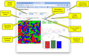
This image shows the browser window running the sample individual-based site "Rock Paper Scissors". The features are all described later in this guide.
- Model Inputs
- These sliders set parameters for the simulation. Changes are forwarded even while the simulation is running and may have immediate effect.
- Timers
- These windows show the current model time. The left window counts up from 0. If the simulation is designed to run for a fixed time period, the right timer window will be initialized to that time and will count down.
- Operating Buttons
- The Connect/Disconnect buttons activate/deactivate the connection between the UI and the model logic. Disconnecting and Connecting is one way to restart the application; reloading the page is another.
- The Reset, Step and Start/Stop buttons operate the simulation. Step executes a single time step, Start/Stop bring about continuous operation, and Reset restores the initial state and resets the timers. Double-clicking Reset also reinitializes the application.
- Speed Control
- This determines the real-time interval between steps.
- Displays
- A spatial or agent-based simulation will include a "SimWorld" display that uses graphic cues to show the current state of the model. Among these cues are location and color, for both cells and agents, and, additionally, size and shape for agents.
- Other displays such as Spys (showing a single current value) graphs, tables, etc. are specified in the Project file (see below).
- Side Panel
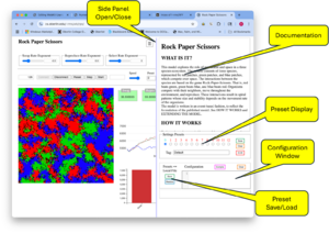
- The browser page has a side panel contained in a "drawer". Use
 to toggle it open and closed, or pull on the lavender bar to adjust its location. The drawer contains model documentation, the preset display, a configuration window, and a log window for status reports. If the site uses RAMs the side panel will be wider and will contain access to RAM controls.
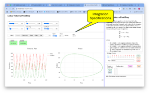
- System Dynamics
- The third image shows the model library SD Lotka-Volterra site. An SD site will display the current choices for dt and integration method (Euler or RK4). These can be overridden from factory settings using the configuration window.
In subsequent sections we describe the platform's features with illustrations using one or more of the sites in the model library. The full model library can be found in the WebKit Examples document. Note that we will be looking at the Javascript model implementation only at this time, as some of the features described here are only available with this implementation.
When opening the Model Library examples you are advised to right-click and open the link in a new tab.
Among the topics covered are:
- User initialization of spatial and agent-based models
- Presets
- NumML language
- RAMS and URAMS
- Configuration overrides
- Analysis platforms
- Downloading CSVs
Model Initialization and Using Presets with Conway's Game of Life and Agents (1)
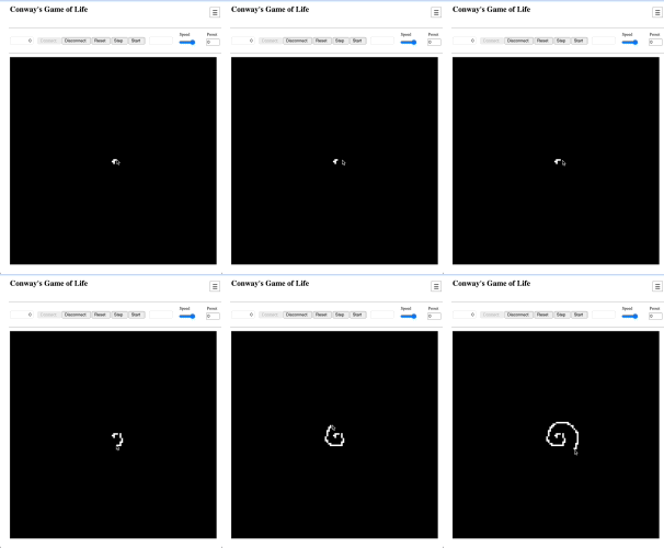
Conway's Game of Life (CGOL) uses a 128 x 128 board with solid edge and an initial configuration consisting of the "R-pentomino". (Try it!) CGOL's model operates on a cellular automaton with 2 possible states, dead and alive.
Agents is a very simple simulation of agents of different sizes and shapes. The space in which they are moving has elastic walls off of which the agents bounce. They also behave like an ideal gas with respect to their physical interaction. (This behavior was a choice made by the site's author.) Agents (1) has the same model, only initially empty.
With NWK you can:
- Click and drag to create new initial configurations;
- Save your configuration in the Presets.
Creating new initial configurations in CGOL
This CGOL simulation uses a Cell Matrix with black/white respectively representing dead/alive. To alter the initial configuration, press or click the left mouse button on any black or white cell to toggle that cell to the opposite color. If you press the mouse button, you can drag the mouse to change dragged-over cells to the new color.
When done, click the Reset button once; clicking Run will execute the simulation with the new configuration, and single clicks on Reset will restore your initial configuration. Double-clicking Reset restores factory settings.
Creating new initial configurations in Agents (1)
You add agents to Agents (1)'s landscape in a similar manner. Shift-click on a cell to add an agent, and continue to shift-click to rotate through cell colors. At the end of the rotation the agent will be deleted. You can also delete an agent immediately with alt-shift-click.
When done, double-click Reset, and then Run. To restore factory settings you must reload the page.
Preset Basics
The Preset feature provides a quick way to save and restore a configuration, modeled on the "radio buttons" found in cars. The Preset control consists of 13 such preset buttons. Each preset label is either red or green, respectively, depending on whether or not the preset is currently assigned to a configuration. Selecting a "green" label will restore the configuration saved in that preset. Selecting a red label has no effect on the configuration.
Note that preset 0 is permanently bound to factory settings and cannot be changed.
Tags. Each preset can be optionally given a tag; i.e., a label used to identify the settings for that preset. Simply enter the tag in the Tag text field before saving the preset.
Preset and tag selection are also controlled from the main control panel, making it unnecessary to have the drawer open while shifting between different presets. The Preset control is located to the right of the Speed slider, and rotates through the available presets as it is clicked up or down. Tagged presets display their tag when selected.
Configurations are saved and cleared using the Save/Clear/Cl All buttons to the right of the Preset controls. Whichever preset is selected will be affected by Save/Clear; Cl All will delete all presets (except for preset 0).
Presets are stored in the Web browser and will be there when you return to the site. A local JSON file storing the complete current bank of presets is created using the Preset ↔ Local File controls found to the left of the Configuration window. Use stored presets as a backup, for transferring between browsers, and when you exceed the 12 user preset limit.
Something to try
Create a set of CGOL and Agent (1) initial configurations using the mouse as described and store them in presets. Test the presets by restoring the configurations. Practice using Save and Clear until you are comfortable with building configurations and storing/restoring them using the presets.
One more thing about Presets
Some site include ready-made presets. These will be installed the first time you access the site. You may make changes to and save ready made presets. You can restore the factory set of ready-mades by deleting all presets and reloading the site.
Using RAMs with the Extended Game of Life 3 (EGOL3)
RAMs provide the means for changing some aspect of the site's model. Each RAM presents a set of alternatives, including a Display or Default alternative that is part of the factory settings. An Alternative may require some additional input through sliders, text fields or text areas. Space is provided so that RAMs are thoroughly documented.
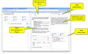
EGOL3 is an extension to Conway's Game of Life to 3 live states (birth, newborn and adult). The simulation has been constructed to support 4 alternate approaches to the creating the initial state, which are presented to you as a RAM with 4 alternatives. The RAM is revealed when the drawer is fully open and Initial State is selected from the RAM Selection Panel (see right).
The RAM Selection Panel appears whenever a site contains one or more RAMs. Selecting a RAM replaces the content of the Documentation Window with overview documentation for the selected RAM. A new column appears topped by the RAM Alternative Selection Panel. Each alternative introduces documentation specific to that alternative and, if needed, a set of input controls (in some cases an input control such as a text area is included for reference only and cannot be edited).
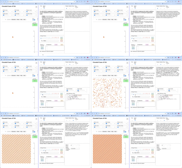
RAMs are powerful tools when combined with presets since the selected RAM and any input values are stored as part of the preset configuration. The factory settings for EGOL3 include 7 different initialization configurations realized mixing different main parameters, RAM alternatives and RAM parameters. You can see this in action by opening the RAM panels as shown and clicking through the 7 presets, as shown at right.
The Display RAM setting is analogous to the conventional GOL we explored earlier. You can set your own initial configuration through click and drag like before. The Random setting lets you choose the probabilities for initial live cells. Reg6 and Reg Custom produce diagonal stripes that repeat with, respectively, a fixed interval of 6 or with an interval between 2 and 12.
Something to try
Make changes to the existing presets. When editing a textfield input, be sure to hit Enter when you are ready to register the change. Save configurations in any of the remaining empty presets, or override the factory presets (except for Preset 0).
When you are done you can restore the initial preset configuration by deleting all presets with Cl All and then reloading.
Using RAMs with the Deterministic SIRS w/ Vaccination (SIRS)
SIRS is rich with RAMs with one (Immune to Vaccinated) containing an alternative (User Input) requiring code. This alternative lets you program how individuals in class R (recovering) are vaccinated and transferred to class V (vaccinated), as a function of model time. A set of variables that can be referenced in the code is provided.
An example is contained in Preset 1. Here we choose to use apply the vaccination rate from the vaccination onset time (both set with the main input sliders) to a time determined using the RAM slider User 1. In other words, you add a shut-off time for vaccinations which has not been provided by the original model. Other possibilities for this RAM could be, for example, to let the vaccination rate decay to account for depletion of vaccine, using the User 1 slider to determine the decay rate.
The code used in Preset 1 is Javascript. Press the Compile button when your are ready. The Enlarge button opens a browser-wide editor window, making code entry easier. If you want to try your own User Input RAM, be sure to save in a preset or your code will be lost.
User-Defined Models (URAMs) with Sensitivity Analysis
The RAM interface makes it possible to easily implement SD simulations defined entirely by the user. An example from the model library containing 4 user-defined presets is SD User Defined.
Such sites are initially defined only by the input and output components they support. Their operation relies on a user-defined program, specifying the model and its UI, that is entered using a RAM. The example site has a RAM with one option, that option showing a text area for the program. It also provides sufficient input and output components to support the UI needs of models implemented on the site.
The example site includes 6 slider inputs, a line graph and a phase graph. Each of these 8 components need a "handle", an ID by which they can be referenced in the program. The sliders all run from 0 to 1 with 0.01 step size and have the IDs Param1, Param2..., Param6. The line and phase graphs are respectively given IDs mainGraph and phaseGraph.
Visit the model using the link and open the Model Definition RAM. It contains a single option (NumML Code) with a Code text area. Notice that, although 6 sliders were allotted, only 1 is visible in the default preset. This is a result of the UI configuration contained in the program. As you step through presets note that the input sliders appear and disappear as needed, and that slider and graph legends (names and titles) change to suit the model.
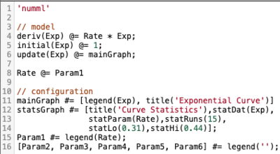
Consider the code for the default Exponential Curve model:
The first line consists of the string "numml". This is required to indicate that the contents are in NumML rather than Javascript. There are 2 sections: model and configurations. (Note that "//" is the comment character meaning that this line is ignored by the compiler). In the model section are 4 statements using the operator @=. In fact, each NumML statement uses Javascript syntax, but with 2 non-Javascript operators: @= and #=, which completely program the behavior and look and feel of the simulation. The former is used to specify the model generally in terms of differential (or difference) equations using program variables; the latter asserts properties for the visual components that fit with the particular model
The first block (lines 4 - 8) consists of 3 statements defining the variable of interest, Exp, and one defining an auxiliary variable Rate used in line 4. The latter is not entirely necessary; we could instead have written line 4 as deriv(Exp) @= Param1 * Exp, however the style we used relates the model directly to relabeling of the Param1 slider to Rate and consequently is more readable. We will continue to see this approach used in the other models in this site.
deriv(Exp) specifies a differential equation on line 4 relating Exp to itself and local variable Rate. Line 8 binds Rate to Param1, which is the alias we assign to Param1 on line 14. Line 5 provides an initial value for Exp, and line 6 links Exp with the line graph mainGraph, which displays its output..
Lines 11 through 16 use operator #= to detail the appearance of the input sliders and output graphs. This is mostly self- explanatory, except for the entry for statsGraph, which will be discussed below. This code is not required, however the result will be a generic display with 6 input sliders labeled Param1 through Param6, and graphs with no labels. Note that on line 16, setting the legend for the unused sliders to an empty string hides them.
Look at the remaining preset code. Preset 3, in particular, is a good example of the extent to which input sliders can be detailed. This is required because the generic slider properties do not match the value range required in the simulation. Refer to the NumML Language Reference for a complete description of the NumML language.
If you make changes to any of these that you want to save to presets, you should compile before saving so that the compiled code will be loaded when you activate the preset.
Sensitivity Analysis
One of the goals of NWK is to provide secondary platforms for optimization and analysis. To date one such platform exists to perform sensitivity analysis, primarily but not exclusively for SD models. Once again, refer to SD User Defined to see this in action. Open this site and click on the tab labeled Sensitivity.
The figure show on the right shows the Sensitivity Analysis platform for the logistic model (Preset 1) after a run. There are 4 user parameters that govern the behavior as shown:
- Parameter: which parameter is varied (in this model it is Rate).
- Runs: how many runs (20);
- From: initial value (0.25);
- To: final value (0.54);
Clicking Start initiates 20 runs with the Rate parameter uniformly stepping through intermediate values between 0.25 and 0.54. During this run, clicking Stop allows the most recent run to finish, allowing the process to continue by subsequently clicking Start. Alternatively, clicking Step proceeds one run at a time until the process concludes. Double-clicking Reset reinitializes the run.
Results are displayed on 2 graphs, the first being identical to the one on the Run platform. To its right is a graph showing mean ± standard deviation of the point-wise variations seen in the run.
Now open the Model Definition RAM and look at the code in lines 12 - 15 to see how the Sensitivity Analysis platform was programmed. The statistics display has ID statsGraph. In addition to specifying a title ("Logistic Statistics"), we see the following entries:
- statDat(N)
- N is output variable of interest
- statParam(Rate)
- Rate is the input parameter to be varied
- statRuns(20), statLo(0.25), statHi(0.54)
- 20 runs with Rate varying uniformly between 0.25 and 0.54
Note that except for statDat, these settings are shown in textfields and merely initialize their parameters. They can be changed, and changes are saved to presets.
Configuration Overrides
NumML statements using #= can be used to configure most models using the Configuration window below the Preset selection window. Shown at right is an override of the factory settings that changes the dt value and asserts Euler as the integration method. Other overrides will become available soon.
CSV Downloads
If a graph contains a CSV button, clicking that button once the graph has been filled will bring about a download of a CSV (comma separate values) file of the data from that graph. The settings used by the simulation will be recorded above the CSV header.
- ↑ This API is under development.
