Pop1

This very simple Ramp introduces the advanced features.

Obtaining Pop1

Fig 1. Studio after installing Pop1

1. Download the file Pop1.xml from here.
2. Launch Numerus Studio and select the File | Open Ramp(s)...; navigate to the folder containing Pop.xml and select it.
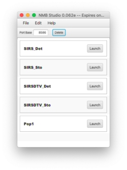
3. When you are done Pop1 should appear on the Numerus Studio dashboard. (Fig. 1)

"Discovering" Pop1

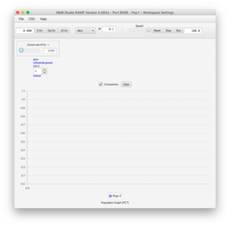
1. Launch Pop1, resulting in the application shown here:

Fig 2. Pop1 Ramp

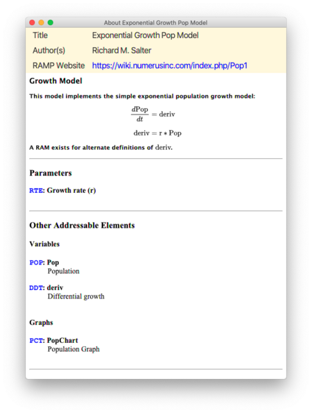
2. Open Help | About This Ramp... to learn about the model and its structure, as shown here:

Fig 3. Pop1 Documentation

The document provides a description of the model and its salient parameters, variables, etc.; use this to familiarize yourself with the model. A link appearing in the title section will lead to more in-depth documentation.

3. You now have an opportunity to test what you learn from the documentation by possibly running the simulation several times with different parameter values.

Fig 3. Pop1 Documentation

Using RAMs

The documentation points out that a RAM exists for overriding the default definition of deriv.

4. Visit the RAM page either by double-clicking on the blue text of the RAM entry, or by clicking the Op On/Off button.

Fig 4. RAM Management Portal

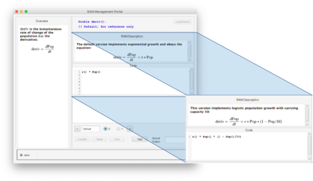
The RAM portal gives a general description of the model variable and shows and describes each of 2 alternatives. The first (default) implements exponential and the second logistic growth. Both use parameter r as growth rate; the second has a fixed carrying capacity of 50. It is apparent that the code used to implement these two models closely follow the equations; note, however, that each element appears as a function of 0 arguments. This is the standard approach used for coding in the Numerus Designer.

A definition in red indicates that the code has not yet been compiled; i.e., translated into runnable form. The default RAM is compiled when the Ramp is launched. Clicking the compile button performs this translation on override RAMs, following which the new version of the model is ready for use. Compilation of RAMs is generally handled automatically when you first click the Reset button before running the model with a RAM other than the default.

You may add your own RAM to the set by clicking on the + button. As a point of departure you can insert the default definition by clicking the Default button. You should make sure that your code compiles before attempting to use it. You can also test the RAM directly with the Test button, and compare its result with a test of the default RAM and any other defined RAM. A keyword entered here will appear on the RAM dashboard to remind you of the change in the model brought about by the RAM. You can also include your own documentation in plain text above the definition.

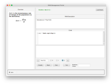
Here is a new RAM that defines the derivative as r * Pop^1/2.

Fig 4. RAM Management Portal

When you are ready to proceed, close the RAM portal. The RAM selection dashboard uses a spinner to select the RAM to be used in the next run. It also shows the keyword associated with the RAM and its status (red for uncompiled, green for compiled.) Never run a model showing a red RAM in the dashboard. Clicking the Reset button will attempt to compile the RAM. If the dashboard entry remains red, then the RAM contains errors and should be fixed.

RPL Scripting

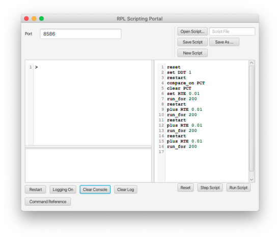
5. Open the Scripting Portal using the button S On/Off. It contains the following script:

Let's consider each entry in the script:

reset

Resets the simulator; this should be the first statement of any script.

set DDT 1

DDT is the airport code for the deriv RAM. Index 1 is assigned to the logistic growth model.

restart

This command needs to follow the change in model. It re-initializes the simulation.

compare_on PCT

Sets the graph (airport code PCT) to comparison mode, in case it wasn't already.

clear PCT

Empties the graph of earlier runs, if necessary.

set RTE 0.01

Initializes the rate parameter (RTE) to 0.01

run_for 200

Executes the simulation for 200 steps.

restart

plus RTE 0.01

run_for 200

restart clears the simulation without returning the parameters to their pre-script values;
plus RTE 0.01 increments the rate parameter;
run_for 200 runs with the new settings for 200 steps.
This sequence is repeated 4 times.

Try running the script. Turning on logging shows each command as it is executed. You can also try stepping through the script line by line.

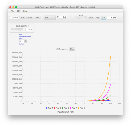
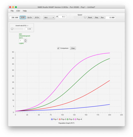
The result of running the script is shown below:

Exercise: What single change do you have to make to the script to produce similar results using the exponential growth model?

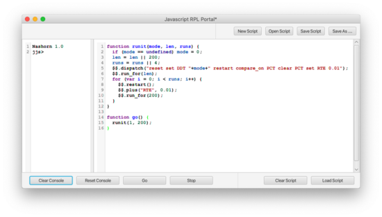
Using Javascript

Javascript is an important programming language used extensively for scripting Web applications. Numerus Studio includes a Javascript runtime engine for executing more sophisticated scripts than can easily be run using the RPL portal directly. The latter is useful when developing in Javascript to test various RPL codes before incorporating them in a full Javascript program.

Opening the Javascript portal you will find a program designed to accomplish the same task as our previous example, but more expressive in several ways. First, instead of necessarily repeating lines of code in the RPL example to perform the same task with a different rate parameter, we use a looping structure (lines 6 through 10). Secondly, we make the program a function into which we pass parameters mode len and runs; the former is either 0 or 1, depending on whether we want to use exponential or logistic growth. The second, determines the length of the run, and the third the number of runs. If these parameters are omitted, the program defaults to exponential growth with a runtime of 200 and 4 runs. Notice that the same set of RPL commands is used (accessed through the $$ object) as in the direct RPL version.

Our go function, which facilitates a default operation, is set up to run identically to the RPL script.

This program also illustrates the two ways one can reference RPL commands from Javascript, using the $$ object. Line 4 shows a call to $$.dispatch containing a sequence of initializing RPL commands represented in a single string. Lines 5 and 7-9 call individual RPL operators using their equivalent $$ entries.

Exercise: run different variations of this program by typing runit(...) with different values for mode, len and runs.