Gradient

In this tutorial we will consider a system in which some currency is transferred from one stock to another in a manner that is dependent on some diffusion constant K multiplied by the difference in concentration between the two stocks. Thus, this is ultimately a model of diffusion, and this formulation can be applied to many kinds of natural phenomena.

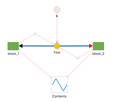
First, we will need two stocks, let”s call them stock_1 and stock_2. You can imagine any kind of currency within these stocks: ions, water, nutrients, etc. Let”s set the initial conditions as stock_1 = 100 and stock_2 = 500. Place stock_2 to the right of stock_1, but be sure to leave space for a flow in between them.

Now we will need a flow connecting the two stocks. For the sake of this model, we will just name it flow and you can imagine this flow as any number of paths or processes: the vasculature of a plant, an ion channel on a cell, and so on. Since this is the thing carrying our currency from one stock to another, it is quite analogous to vasculature or other mechanisms of nutrient transfer in living things. In this case, this flow should be a biflow, because the currency can diffuse in either direction depending on the gradient. Connect the clouds of this biflow to each stock.

Next, we”ll need a diffusion constant. Drag out a term and name this constant K, and we”ll say it has a value of 0.3.

Now we need to configure the equation within our flow. Use connectors to connect both stocks and K to the flow. Now, view the flow's properties and set the equation to be K*(stock_1-stock2). Since this is a biflow, if the difference is positive (if stock_1 > stock_2) it will diffuse in the forward direction, and if the difference is negative (stock_2 > stock_1), it will diffuse in the backward direction.

Now lets make a graph to visually represent changes in stocks 1 and 2. Drag a LineGraph onto the canvas and name it Contents. Select stocks 1 and 2 to be graphed in the time series.

Your model should now be ready to run, and should look something like this:

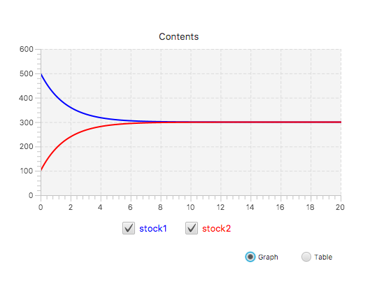
We are ready to run the model. Click launch, then run, and graphical output should be visible on your graph. Notice how the two stocks meet in the middle at 300? Your stocks have reached equilibrium, and your graph should look something like this: