Overview

The SEIVAgent Simulator is software to accompany Getz, et. al.,Adaptive vaccination may be needed to eliminate COVID-19: Results from a runtime-alterable strain-drift and waning-immunity model, https://doi.org/10.1101/2021.06.07.21258504. Complete documentation for the application is contained in the latter. This User Guide provides general instructions for using the program, together with some example runs from the paper.

Using SEIVAgent

SEIVAgent is a stochastic model simulating an epidemic spreading over a population of individuals over some time period. Individuals states include S (susceptible), E (exposed), I (infectious), V (vaccinated, recovered) and D (dead). A set of 18 parameters govern the epidemic over a course of time units (days, weeks, etc.)

Individuals are contained in one of three different compartments or pools. At the start of the program all individuals but one are part of the susceptible pool. Individuals in the susceptible pool remain anonymous and this pool is tracked only in terms of its size. As the algorithm progresses through time, individuals in state I can infect other susceptible (state S) and recovered (state V) individuals. Once exposed, an individual enters state E, becomes part of the identified pool if not already there, and progresses through states I and either V or D. If the individual enters state D it is removed from the experience pool and enters the dead pool.

The program models both the initial infection and emerging variants. Each individual is currently in some state with respect to each of the variants. Variants are numbered 0 to 2^J - 1 for some fixed integer J.

SEIVAgent is initialed with a given population size N and a single individual in state I with respect to the initial strain (variant 0). All other individuals are in state S.

The program executes as a series of time steps. At each time step new susceptible and recovered individuals may be exposed to some strain. Each individual can only be exposed and infected with respect to one single strain at a time. Exposed individuals become infectious and infectious individuals either recover or die.

Governing the progress of individuals through the epidemic are probabilities that are computed using the parameter set. Full details of the algorithm are provided in the paper. Along with these parameters, the user may set up a vaccination protocol, which is governed by parameters contained on the vaccination page (see below).

The program implements some novel features designed to provide expressiveness and promote experimentations. These include an API available for both on-board and remote access. The second feature is a set of runtime alterable modules (RAMs) that manage changes to the basic algorithm in a safe environment.

On start-up, SEIVAgent restores the settings from the previous sessions. Settings may be saved and restored in an XML file. In addition, pathogen settings may be saved independently and used with other parameter sets.

The Main Dashboard

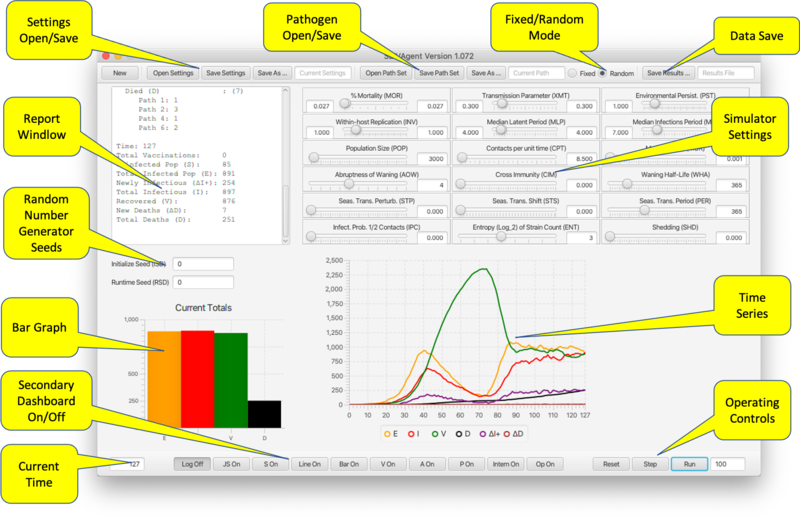
The main dashboard provides sliders for entering parameters, controls for operating the program, and output in the form of graphs and a current status report. It also provides controls for viewing the secondary frames containing additional graphs; pathogen settings; vaccination settings and status; agent status; API access; and RAM management.

Settings Open/Save. The simulator always opens in same state it was in at the end of the last session. Current settings are saved at any time to an XML file for subsequent reloading. Settings include all parameters, vaccination settings and pathogen properties.
Pathogen Open/Save. Saves pathogen properties for subsequent reloading, in particular for use with a different set of parameter/vaccine settings.
Fixed/Random Mode. In Random mode, on Reset the six pathogen parameters (environmental persistence, transmission, within-host reproduction, and disease-induced mortality rates, as well as shedding and cross-immunity matrix values) are chosen randomly from the ranges set with range sliders (see below). In fixed mode a Reset does not change the pathogen parameters. Loading a pathogen file (previous bullet point) triggers Fixed mode.
Data Save. Saves the results of a run to a comma-separated-values file for use in a spreadsheet.
Report Window. Shows the changes occurring over the most resent time step.
Random Number Generator Seeds. Seed values for separate RNGs used to select parameters and during runtime. If left blank RNGs operate unseeded.
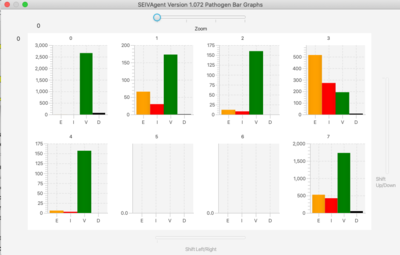
Bar Graph. Shows the current state (SEID) of the total population.
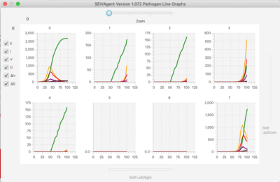
Time Series. Shows the evolution over time of the state of the population (SEIV together with ΔI+ representing positive change in the infectious population—i.e. incidence, and ΔD representing number of deaths from disease in the last time period).
Operating Controls. Reset, Step, and Run. The latter requires the number of steps to be entered in the textfield. The number in the textfield will count down as the program traverses the time steps. Run can be interrupted and continued to the end of the number of prescribed steps.
Secondary Dashboard On/Off. Opens/closes secondary dashboards and viewers(described below). These include:
- Line On/Off, Bar On/Off. Time series and bar population graphs broken down by pathogen.
- V On/Off. Vaccine Viewer.
- P On/Off. Pathogen Viewer.
- A On/Off. Agent Viewer.
- Intern On/Off. Internal Values Display.
- Op On/Off. RAM Operator Redefinition Frame.
- S On/Off. Direct API Scripting and Monitoring.
- JS On/Off. Javascript API Scripting.
- Log Off/On. Disables Report Window reporting.
Simulator Settings. Below is a table associating sliders to parameters described in Table 1 in the paper:

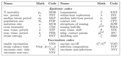
% Mortality* (MOR)	α
Transmission Parameter* (XMT)	β
Environmental Persist.* (PST)	η
Within-host Replication* (INV)	λ
Median Latent Period* (MLP)	σ_E
Median Infections Period* (MIP)	σ_I
Population Size (POP)	`N₀`
Contacts per unit time (CPT)	κ
Mutation Rate (MUR)	μ
Abruptness of Waning (AOW)	σ
Cross immunity (CIM)	c_i,j
Waning Half-Life (WHA)	t^half
Seas. Trans. Perturb. (STP)	δ
Seas. Trans Shift (STS)	θ
Seas. Trans Period (PER)	k
Infect. Prob. 1/2 Contacts (IPC)	p^half
Entropy (log₂) of Strain Count (ENT)	n
Shedding (SHD)	ζ

The three-letter "airport codes" are used to reference these parameters from the API. The *-ed parameters are range values for pathogen settings from which a parameter value is selected if operating in Random Mode. Ranges can be eliminated by setting the top and bottom range endpoints to be the same.

Other Viewers

Internals

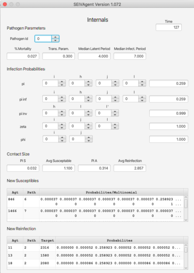
The Internals dashboard displays various internal values for verification of the algorithm with respect to selected parameters. The top section (Pathogen Parameters) can also be viewed on the Pathogen dashboard. The terms pi, pi inf, etc. refer to probability functions discussed in the paper. The argument spinners can be changed to compute the functions for different input values. Similarly, Pi S and Pi A refer to probabilites related to contact size. The bottom pair of tables break down the probabilities with respect to pathogen strain.

This dashboard is particularly useful when using the RAM feature as a means of verifying RAM redefinitions.

Pathogen and Agent Viewers

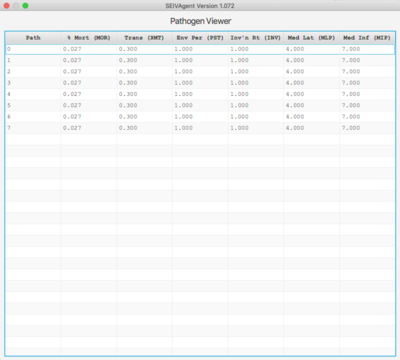
The Pathogen viewer displays the current pathogen set and each pathogen's 6 defining parameters. Double-clicking on an entry allows the entry to be edited. The entire pathogen set can be saved an associated with a different set of general/vaccine parameters.

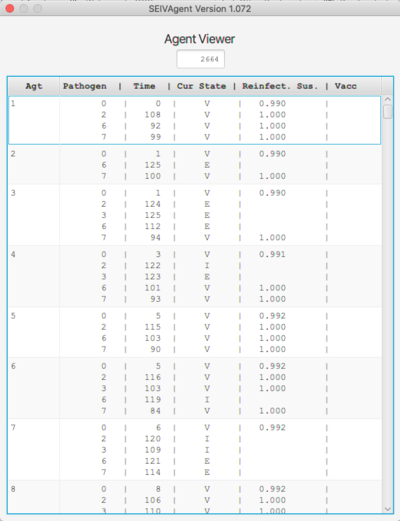
The Agent viewer shows the current state of the agent set. Only those agents who have been infected at some point and are still alive are shown. For each agent and each pathogen infecting that agent, the time of infection, the current state and reinfection probability are shown. If the agent has been vaccinated for a given strain, the state of the agent at the time of vaccination is also shown.

Vaccination Viewer

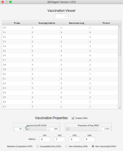
The Vaccination viewer shows the number of individuals vaccinated at each time step, broken down by their state at the time of vaccination (either S or V). The bottom of the viewer contains inputs that determine the vaccination protocol. These are:

Enable (VEN). Vaccinations take place only if this is checked.
Vaccine On/Off (VOO). Sets the time period during which vaccinations will occur.
Proportion of Pop (PRO). Sets the probabilistic mean for selecting vaccination candidates.
Valency. The vaccine can be effective for up to 4 strains (if fewer, leave those textfields blank.)
Selection Composition (VCP). Three different protocols are available:
- Susceptible Only (VSU). Candidates are drawn only from the susceptible pool.
- Non-Infectious (VNI). Candidates are drawn from the susceptible pool and agents who are currently non-infectious (i.e., not in state I for any strain).
- Non-Vaccinated (VNV). Any non-vaccinated individual can receive the vaccine.

In the latter two cases, candidates are drawn in proportion from each pool (susceptible and identified) in proportion to the size of the pool.

Graphs

The simulator has a lattice of line graphs, one for each variant, showing the time evolution of the population in each state. Graph overlays of interest are selected using checkboxes. There is a similar lattice of bar graphs showing the current population in each state for each variant.

For very large variant sets, a zoom feature focuses the display on only one section of the graph lattice. Sliders to shift the view to different sections of the lattice appear on right and bottom margins.

Simulator Operation

The three buttons on lower right button bar operate the simulator:

Reset. Sets the time to 0 and returns the simulator to the initial state. In Random mode, new parameter values are selected for pathogens from their assigned ranges (in Fixed mode the parameters remain as they were in the previous simulation).
Step. Executes a single time step.
Run. If a number is present in the textfield the simulator begins running for that number of steps. The textfield counts down as each step if completed. The Run button is a toggle; if it is pressed while the simulator is running it will curtail the execution after completion of the current step. It may be pressed again after stopping to continue the run from the stopping point. Reset always restores the run count to its original value.

Saving Results

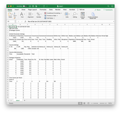
Clicking the Save Results... button brings up a file chooser with which you select a CSV file to contain the data record of a simulation run. Part of this file is shown here in Excel. The CSV file contains the following sections:

Parameter Settings. Based on slider entries.
Vaccine Settings. If enabled, contains same information as the bottom of the Vaccine viewer.
Vaccine Administration. If vaccines are enabled, contains same time series information as the top of the Vaccine viewer.
Pathogen Properties. Same information as the Pathogen viewer.
Time Course per Strain. Data recorded in the per-strain line graphs.
Totals. Data recorded in the dashboard line graph.

Mid-course changes made using the API are made clear in the data record.

API

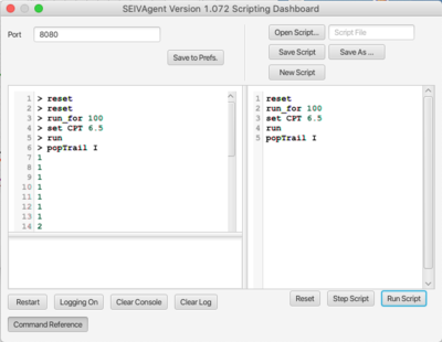
The simulator API is a simple bytecode called BPL (Blackbox Programming Language) that addresses all available user interactions with the simulator. Instructions fall into three categories: parameter assignment and retrieval; simulator operation; and data retrieval. A complete list of instructions can be obtained by pressing Command Reference button shown on the API Scripting Dashboard at right.

Instructions are comprised of opcodes (e.g.,reset, step, get) followed by 0 or more arguments. Every BPL operation returns a result, even if empty, for synchronization purposes. A string consisting of a sequence of opcodes and arguments may be submitted to the BPL interpreter, an example of which is shown here.

Parameter assignment and retrieval. Every user-configurable element (including random number generator seeds) is addressed from BPL using a unique three-letter “airport code” as shown at right. Additionally, pathogens are addressed by their id number (0 to 2^J−1) and agent states using identifiers S, E, I, V, DI+ and DD (the latter two represent ∆I and ∆D, respectively). RAM options are addressed using the name of the RAM (e.g., “crossImmune”). Get and set operations can be used on each of these with the exception of ENT (strain entropy), which is read-only.

Simulator operation. Simulation runs begin by executing the BPL reset instruction, followed by step, run_for or run. The BPL interpreter operates synchronously with the simulator by waiting to process subsequent commands during a simulation run. Operational instructions can be interspersed with parameter set/get or data retrieval to use in runtime decision-making. Note that the reset operation restores the simulator to its state at the time of the last reset, so that no parameter changes made during a run are persistent.

Data retrieval. Operations to obtain the current population in each state, and to retrieve the runtime population history of each state and pathogen are also included. These can be easily transformed into R ^[1] data frames, for example, for further analysis.

Scripting can be deployed using either one of the two on-board script interpreter interfaces, or remotely from another platform using drivers provided with the simulator. The remote drivers use TCP/IP sockets. In this case the simulator acts as a server fielding API requests from the remote drivers.

API Scripting Dashboard

The API scripting dashboard (shown above) is intended as a development platform for scripts, and for monitoring the behavior of remote scripts during execution. A short script is shown in the right-hand script pane. Scripts can be single-stepped or run completely using the buttons on the bottom. The left-hand console pane contains an interpreter into which script statements can be entered and executed. The Reset button resets both the console and script pane. Single-stepping copies a single line from the script pane to the console and executes it. Note that the scripting system does not report errors, but rather returns in an empty reply, so that it is wise to check the behavior of scripts carefully before deploying. Other controls include:

Restart Reinitializes the script interpreter.
Logging On/Off When logging is enabled remote execution of script statements are logged in the lower-left text area.
Clear Console Erases the console without resetting or reinitializing.
Clear Log Clears the log text area.

Javascript Console

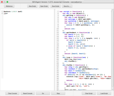
The Javascript console presents an interactive Javascript window (left) and a script development window (right). The Javascript interpreter has been extended with an SEIV object containing methods corresponding all of the the API opcodes. Complete documentation is contained in the Javascript Console Reference, which can viewed by clicking the Reference button.

The SEIVAgent distribution contains a sample script vacadjust.js, which implements the following protocol over a multistrain simulation with vaccinations enabled:

script(n, m, d)

Run for d time units
Determine the strains with the 2 highest populations of infectious individuals.
Vaccinate for those 2 strains for m time units.
Repeat steps 2 & 3 for a total of n time units.

Remote API Access: Using SEIVAgent with R

The API supports remote control of the simulator from independent platforms using the operating system’s socket interface. The simulator's server listens on port 8080 (or whatever port is entered into the Port textfield on the Scripting dashboard, followed by Restart) for clients transmitting an API command string, whereby the server replies with the result. Client software for other language platforms (Python, etc.) can be easily configured using their intrinsic socket architecture.

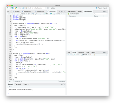
Of particular interest is integration with the R statistical programming environment. An R-package called “seiv” distributed with the simulator acts as a driver by synchronously issuing BPL command strings and waiting for results. Consequently, a simulation can be driven entirely from within the R platform, treating the simulator as a “virtual package”. The figure at right shows part of the code used to run the simulator multiple times with different random number generator seeds. Following each run, the time history of the population in the I, ΔI+ and ΔD states is extracted directly to an R data frame At the end of the run sequence the data frame is used to build a set of plots.

Runtime Alternative Modules (RAMs)

[Note: this section makes extensive reference to the document contained at https://doi.org/10.1101/2021.06.07.21258504/]

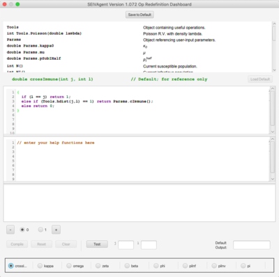
At right is the RAM redefinition frame. The available RAMs appear as radio buttons along the bottom of the frame. Each RAM is a set of options for defining a relatively short Java method implementing some key aspect of the simulation algorithm. Included in this simulation are the implementation for cross immunity given in Eq. 1 of the paper; the implementation for β given in Eq. A.14; and the implementation for φ given in Eq. A.11; etc. Each RAM initially contains only a single option, Option 0, the default, internally defined implementation. Option 0 cannot be edited and appears for reference purposes only.

Additional options may be added to each RAM containing code redefining the method. Two editor panes and one console pane are stacked in the frame and display the code and output of the RAM. These panes show the content associated with the currently selected RAM and option. The top editor pane contains the code for the method being redefined. The second editor pane contains definitions of any new help functions required by the definition in the top pane. The console pane contains messages and output that are useful during the development of the option. For convenience, a “Load Default” button initializes the editor to an editable version of the Option 0 default to use as a starting point.

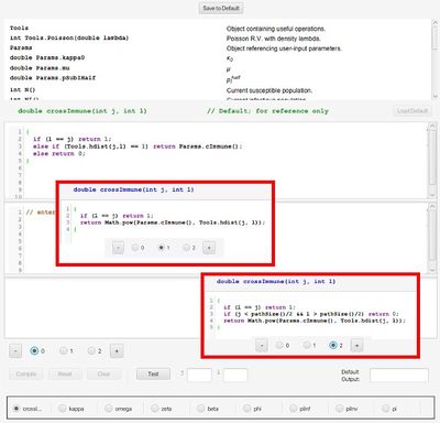
The figure on the right shows the Option 0 default definition for the cross immunity matrix function, as described by Eq. 1. Clicking the “+” button produced two new options, which appear in the insets. These option implement the alternative489cascading cross immunity schemes presented in Eqs. A.7 and A.9. Option 2 code appears below:

double crossImmune(int j, int k) {
 if (l == j) return 1;
 if (j < pathSize()/2 && l > pathSize()/2) return 0;
 return Math.pow(Params.cImmune(), Tools.hdist(j, l));
}

Note that we have substituted the function pathSize for a hard-coded value of 63. pathSize returns the number of pathogens, allowing us to use this formulation for any choice of entropy. Documentation for pathSize is at the top of the window in the list of available help functions and parameters. There is also more extensive documentation in a separate user guide coming soon.

The platform duplicates a mini-development environment for building alternative definitions. Once code has been entered the Compile button checks the legality of the code and makes it available for use at runtime. Legally compiled code will produce a “Compilation Successful” message. Errors will appear with line numbers if they occur. Once the code is legal, the Test button can be used with actual parameters entered into the small text fields to determine correctness of the code. It is also possible to include print and println statements in the code during development to further check correctness. Output from print statements will appear in the bottom console window. The entire RAM set can be saved and will reappear during subsequent launches of the simulator platform.

To use an alternate RAM definition at runtime simply select the desired option. (Selected options will be restored from a saved RAM set during subsequent launches.) The system will compile any uncompiled code the first time it is accessed. If an error occurs during a runtime compilation an alert will notify the user that the system is returning to the default definition of that RAM. At no time is the internal logic of the program overridden. Finally, RAM option selection is part of the API described in the previous section. This means that a script may run a simulation selecting different options at different points in time, using logic that considers the state of the model.

RAM Development Guide

Equation and other parameter references are contained in the paper.

Cross Immunity (c_{i j})

Definition (Eq. 1)

Default Code

double crossImmune(int l, int j){
  if (l == j) return 1;
  else if (Tools.hdist(j,l) == 1) return Params.cImmune();
  else return 0;
}

Notes

`Tools.hdist(j,l)`	Computes the Hamming distance between pathogen i and pathogen j. This is the number of different alleles.
`Params.cImmune`	The cross immunity constant with airport code CIM.

Kappa (κ)

Definition (Eq. A.10)

Default Code

int kappa(int i) {
  double kappa0 = Params.kappa(); 
  double p_I_half = Params.pSubIHalf();
  double kappa;
  if (p_I_half != 0) {
    double NN = (double)NI()/(double)(N() - ND());
    kappa = (double)kappa0/(1.0 + Math.pow(NN/p_I_half, 2));
  } else kappa = kappa0;
  return Tools.poisson(kappa);
}

Notes

`Params.kappa()`	κ0 (Airport code CPT)
`Params.pSubIHalf()`	p_I^Half (Airport code IPC)
`N()`	Total population (Airport code POP)
`NI()`	Current infectious population
`ND()`	Current dead population
`Tools.poisson(kappa)`	Returns a random value drawn from a Poisson distribution with density `kappa`

Omega (ω)

Definition (Eq. 9)

Default Code

double omega(int i, int j) 
{
  if (i == 0) return 0.0;        // Special case; A_0 never infected
  InfectedAgentState astate = getStateOf(i, j);
  if (astate == null || !(astate instanceof V)) return 0.0;
  double tau =  tau(i,j);
  double sigI = sigmaI(j);
  double sigE = sigmaE(j);
  double timeSinceInfect = tau + sigI + sigE;
  if (time() <= timeSinceInfect) return 1.0;
  return 1/(1 + Math.pow((time() - timeSinceInfect)/tHalf(j), Params.sigma()));
}

Notes

`astate=getStateOf(i, j)`	`astate` is assigned to a Java `InfectedAgentState` object for agent i with respect to pathogen j. `InfectedAgentState` objects can either be state `E`, `I`, `V` or `null` (the latter for never-infected or dead agents.)
`astate == null \|\| !(astate == V)`	`astate` is something other than state `V`.
`tau(i, j)`	τ_{i j}
`sigmaI`	σ_I
`sigmaE`	σ_E
`tHalf(j)`	τ_j^half
`time()`	t
`Params.sigma()`	σ (Airport code AOW)

Zeta (ζ)

Definition (Eq. A.12)

Default Code

double zeta(int i, int j, int l) 
{
  return zetaBar(j,l) * phi(i,l); 
}

Notes

`zetaBar(j,l)`	Defined by the following: double zetaBar(int j, int l){ if (l == j) return 1; else if (Tools.hdist(j,l) == 1) return Params.zeta(); else return 0; }
`phi(i,l)`	See entry for Phi
`Params.zeta()`	Shedding parameter (Airport code SHD)

Beta (β)

Definition (Eq. A.14)

Default Code

double beta(int h, int l) 
{
  return betaBar(l) * phi(h,l); 
}

Notes

`betaBar(l)`	The β value of pathogen l, drawn from the range defined by Airport code XMT.
`phi(i,l)`	See entry for Phi

Phi (φ)

Definition (Eq. A.11)

Default Code

double phi(int i, int j) {
  double ans = 1.0;
  for (int m = 0; m < pathSize(); m++) 
    ans *= (1 - crossImmune(m,j) * omega(i,m)); 
  return ans;
}

Notes

`pathSize()`	The total number of pathogens (2^J-1)
`crossImmune(m,j)`	See entry for CrossImmune
`omega(i,m)`	See entry for Omega

PiInf (π^inf)

Definition (Eq. A.15)

Default Code

double piInf(int i, int h, int j, int l) {
  if (pathSize() == 1) {
    return (1 - Math.exp(-betaBar(0)*(1 - omega(h, 0))));
  }
  double numer = zeta(i,j,l) * eta(l) * beta(h, l); 
  double denom = 0;
  for (int m = 0; m < pathSize(); m++) {
    denom += zeta(i,j,m) * eta(m) * beta(h, m);
  }
  double ans = (numer/denom) * (1 - Math.exp(-numer));
  return ans;    
}

Notes

pathSize() The total number of pathogens (2^J-1)

Math.exp(x, y) x^y

betaBar, beta See entry for Beta

omega See entry for Omega

zeta See entry for Zeta

eta

Defined by equation A.13:

η_l	=	the value assigned to pathogen l from the range with Airport code PST;
δ	=	`Params.delta()` (Airport code STP);
k	=	`Params.period()` (Airport code PER);
θ	=	`Params.theta()` (Airport code STS).

PiInv (π^inv)

Definition (Eq. A.16)

Default Code

double piInv(int h, int l, int lPrime) {
  if (l == lPrime) return 1-Params.mu();
  if (Params.mu() == 0) return 0.0;
  double numer = lambda(lPrime) * phi(h, lPrime);
  double denom = 0.0;
  for (int m = 0; m < pathSize(); m++) 
    if (m != l) denom += lambda(m) * phi(h, m);
  return Params.mu() * numer/denom;
}

Notes

`pathSize()`	The total number of pathogens (2^J-1)
`Params.mu()`	Mutation rate (Airport code MUR)
`lambda(j)`	The value assigned to pathogen j from the range with Airport code INV
`phi`	See entry for Phi

Pi (π)

Definition (Eq. A.17)

Default Code

double piInv(int i, int h, int j, int l) {
  double ans = 0.0;
  for (int m = 0; m < pathSize(); m++) ans += piInf(i,h,j,m) * piInv(h,m,l);
  return ans;
}

Notes

`pathSize()`	The total number of pathogens (2^J-1)
`PiInf`	See entry for PiInf
`PiInv`	See entry for PiInv

Notes

↑ R refers to the R Statistical Language.

[1] R refers to the R Statistical Language.

[1]

SEIVAgent IBM Epidemic Simulator

Overview

Using SEIVAgent

The Main Dashboard

Other Viewers

Internals

Pathogen and Agent Viewers

Vaccination Viewer

Graphs

Simulator Operation

Saving Results

API

API Scripting Dashboard

Javascript Console

Remote API Access: Using SEIVAgent with R

Runtime Alternative Modules (RAMs)

RAM Development Guide

Cross Immunity (ci j)

Definition (Eq. 1)

Default Code

Notes

Kappa (κ)

Definition (Eq. A.10)

Default Code

Notes

Omega (ω)

Definition (Eq. 9)

Default Code

Notes

Zeta (ζ)

Definition (Eq. A.12)

Default Code

Notes

Beta (β)

Definition (Eq. A.14)

Default Code

Notes

Phi (φ)

Definition (Eq. A.11)

Default Code

Notes

PiInf (πinf)

Definition (Eq. A.15)

Default Code

Notes

PiInv (πinv)

Definition (Eq. A.16)

Default Code

Notes

Pi (π)

Definition (Eq. A.17)

Default Code

Notes

Notes

Navigation menu

Search

Cross Immunity (c_{i j})

PiInf (π^inf)

PiInv (π^inv)